
Solana players must learn: JLP APY prediction principle and interest rate trading arbitrage model research
Original author: Sean @seanhu 001 , Founder of RateX
TLDR: This article covers three key areas
1. Understand the nature and stability of JLP: The article introduces the principles of JLP and explains the reasons for stable and high returns.
2. Analysis and forecast of JLP’s APY: By breaking down the components of JLP’s APY (such as revenue sources and TVL), it helps readers understand the factors that affect APY and provides guidance on forecasting short-term and long-term APY trends.
3. JLP Income Trading Strategies: The article introduces a variety of trading strategies, including leveraged income speculation, fixed income investments, and APY-based arbitrage opportunities, providing readers with practical insights into income trading.
4. Learn about RateX, the industry’s first leveraged interest rate trading protocol, and how to effectively use RateX to maximize returns.
Since the beginning of this year, JLP opportunities have been one of the most popular asset types in the Solana ecosystem. Not only does it have high returns, but its value is also very stable. Its ultra-high risk return has made it the preferred asset for many investors in the crypto bear market. This article will help readers understand the core of JLP and tell users how to profit by analyzing and predicting JLP's APY.
1. What is JLP?
JLP is the liquidity pool of Jupiter Perp. The assets in the pool are composed of SOL, WBTC, ETH, USDC, and USDT. The latest composition ratio is as follows.
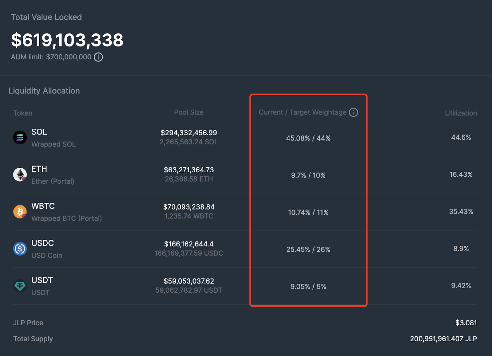
Target Weightage is a goal set by the JUP team and is regulated by setting a Swap Fee or Mint/Redeem Fee.
Current Weightage is the actual asset ratio in the current pool. It can be seen that SOL has the highest ratio of 45%, ETH and WBTC each account for nearly 10%. The remaining 25% and 9% are USDC and USDT respectively.
How to understand the essence of JLP? JLP is essentially a combination of U-standard and currency-standard loan pools. We can divide JLP Pool into 2 parts. The first part is the Crypto part, and the second part is the stablecoin part.
For the Crypto part, there are 3 assets, SOL, ETH and BTC. The role of this part of assets is to lend to Traders for long use. Traders borrow these assets and return the USD value of the borrowed assets at that time. Therefore, for every additional Long crypto transaction in the market, a part of the value of the crypto in JLP becomes a USD loan. When the Utilization of a crypto such as SOL becomes 100%, we can understand that all SOL in JLP has been converted into USD loans.
For the stablecoin part, two types of USD stablecoins are supported: USDC and USDT. The role of this part of assets is to lend to traders for short selling. Traders borrow these dollars and return the crypto amount of the dollar value at the time of borrowing. Therefore, for every additional short crypto transaction in the market, part of the value of the stables in JLP becomes a currency-based loan.
So we can simply get a formula to calculate the real stablecoin ratio of JLP:
The proportion of real stablecoins = the number of real stablecoins / TVL =
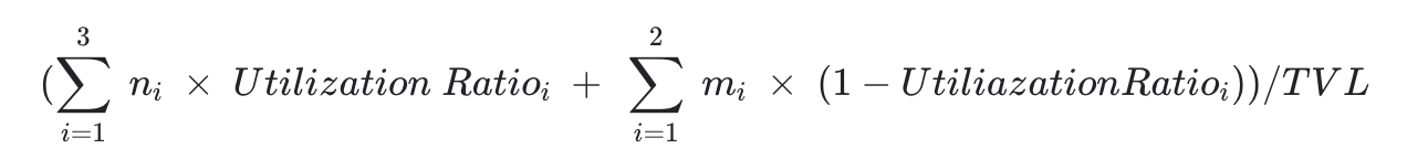
N represents the 3 assets in the crypto part, and m represents the 2 assets in the stablecoin part.
Through this formula, we can see intuitively that when the utilization rate of crypto assets is high (more long positions) and the utilization rate of stables assets is low (few short positions), the value of JLP is closer to a stable currency pool. This means that when the market is bullish, the bulls conduct a large number of leveraged transactions, and the value of JLP is more stable. Of course, JLP will have a certain degree of impermanent loss (that is, the value of the pool is lower than the assets it holds in the bull market, but it is more stable).
On the contrary, when the utilization rate of Crypto assets is low (few long positions) and the utilization rate of stablecoin assets is high (many short positions), the value of JLP is more like a Crypto pool. In other words, in a bear market, if long positions decrease and short positions increase, the value of JLP is more like a crypto portfolio.
Of course, the reality is obviously not what we just mentioned. In the bear market, we see that the proportion of long positions in Jupiter perp is still much greater than the short positions. When I wrote this article (September 5), the long-short ratio still reached 90%.
We can easily get the basic data of the current JLP Pool from here. According to our data analysis, the current real stablecoin accounts for 58.8%. This is also the core reason why we see that the value of JLP is so stable. When there are 60% stablecoins in the portfolio, its value is unlikely to be unstable.
2. How to predict JLP’s APY
Let's look at another interesting point, the income data of JLP, which is reflected in the APY data they push every week. Although JLP is an asset whose income is accumulated in the unit net value, its income is mixed with the fluctuation of the asset value in the pool. However, we can still analyze it through the official APY data or on-chain data to separate the income part from the value of JLP.
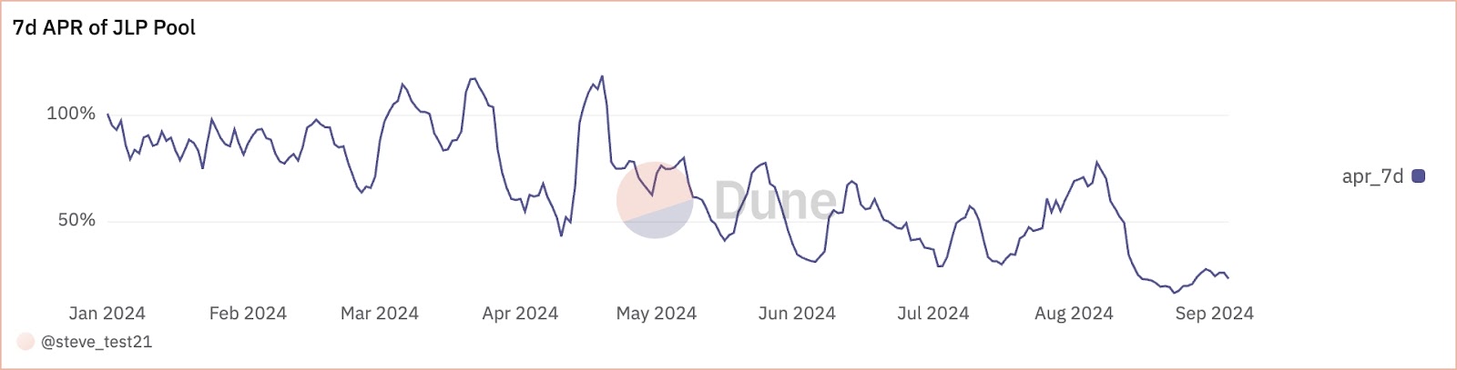
Jupiter does not provide historical APY time series data, but we have made a 7-day average APY curve based on the on-chain data. We can see that JLP's APY continues to be at a very high level of return, and the volatility is also not small. With the gradual expansion of JLP's scale and the market's bearish turn, there is a certain degree of downward trend, but it still remains around 30%.
Next we will analyze the composition of returns in JLP and tell you how to predict the APY trend of JLP in the short and long term.
First, the calculation formula for JLP’s APY is very simple.
APY = Earned Fees / TVL. This section will mainly analyze the earned fees and TVL.
1. Composition of income sources in JLP:
According to Jupiter's official documents, we can see that JLP's revenue comes mainly from the following factors:
The exchange generates fees and yields in various ways:
Opening and Closing Fees of Positions (consisting of the flat and variable price impact fee).
Borrowing Fees of Positions
Trading Fees of the Pool, for spot assets
Minting and burning of JLP
75% of the fees generated by JLP go into the pool.
Thanks to Jupiter, we can see a breakdown of these revenue sources on-chain:
These daily data form the basis of our forecasts for JLP's returns.
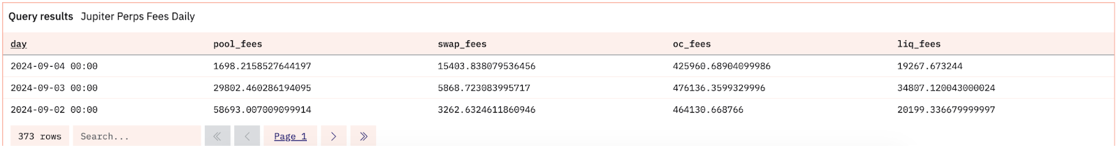
We see that pool_fees corresponds to borrowing fees of the positions, swap_fees corresponds to trading fees of the pool, oc_fees corresponds to opening and closing fees of positions, and liq_fees should correspond to liquidation fees.
https://dune.com/queries/3417634/5738454
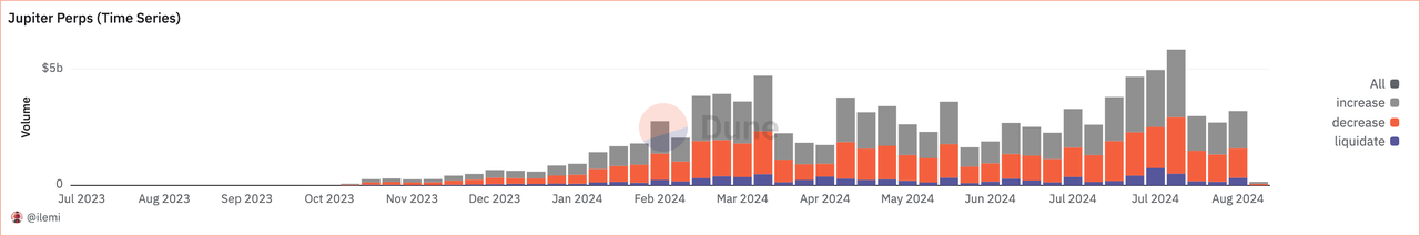
This chart reflects the time series data of Jupiter Perps Fess from July 2023 to the present. We can see that oc_fees occupies an absolute majority, so we mainly study oc_fees.
According to the introduction on Jupiter's official website, Fee calculation for opening and closing positions involves the volume of these transactions, multiplied by the fee percentage of 0.06%. Of course, we know that this fee rate is dynamically adjusted by the official. Assuming that the fee percentage remains unchanged, we know that oc_fees is linearly related to the transaction volume. So as long as we can predict the transaction volume, we can predict oc_fees.
We can get the transaction volume of Jupiter Perps from the chain.
The following figure shows the transaction volume of DEX on Solana
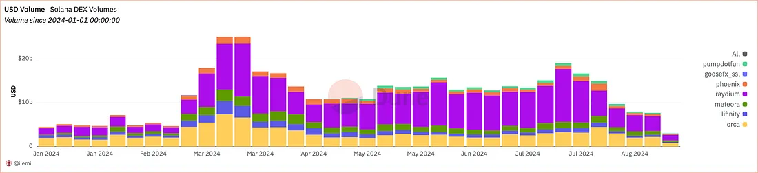
We see that the trading volume of Jupiter Perps is similar to the trading volume of DEX on Solana in trend, but is obviously more independent. While the trading volume has dropped sharply since July, the trading volume of Jupiter Perps has still remained at a good level.
Therefore, when predicting short-term transaction volume, we can accurately obtain Jupiter Perp's transaction data by analyzing on-chain data, but when predicting long-term transaction volume trends, we need to consider both Solana's overall transaction volume trend (beta) and Jupiter Perp's independent growth ability (alpha) as a proven successful project.
2. TVL scale of JLP
After looking at the fee structure, let's look at TVL. This determines how much capital provides leverage and how many people share the benefits with you. We can see from the figure below that JLP's TVL is growing steadily, and the Jupiter team's scale growth strategy for JLP is also relatively stable. They will set an AUM Limit for JLP to control the scale to prevent TVL fluctuations from affecting LP's income, which is a responsible behavior in itself.
https://dune.com/queries/3379693/5670864
In general, as the TVL ceiling of JLP continues to increase, its APY center will inevitably decline. However, considering the current bear market, the market trading volume has dropped by 50% since July. If the market recovers and the competitiveness of Jupiter Perp products, we believe that JLP's APY is likely to rebound within a certain period of time, and it is not impossible to return to a level above 50%-60% APY.
If you want to study short-term APY, for example, get an expected JLP APY before the official APY is announced, you can log in to RateX ’s official website, click JLP contracts in the market overview after the mainnet is launched, and we will provide JLP’s leading APY data for users’ reference.
3. How to profit by predicting JLP’s APY?
If you understand the research method above and think that predicting APY is fun and easy, then you need to read the following content, which will tell you how to make money through RateX’s JLP yield trading function.
1. Leveraged speculation on future APY.
RateX is a leveraged interest rate trading protocol that allows users to trade yield by synthesizing YT-JLP. In short, it creates a liquidity pool for JLP yield trading, and Liquidity Provider deposits JLP into this pool. Based on the deposited JLP, ST-JLP in the form of rebasing is generated for Liquidity Provider.
The amount of ST-JLP is compounded based on the APY data provided by the official platform, ensuring that the value of ST-JLP after the increase based on the APY provided by JLP is the same as the value of JLP. At the same time, based on the deposited JLP, the liquidity provider will mint YT-JLP from the protocol (generally speaking, depositing 1 JLP allows minting 1 YT-JLP).
Based on YT-JLP and ST-JLP, RateX built a YT/ST AMM pool for users. When a trader wants to use leverage to long YT, he deposits a margin (JLP), and the protocol creates ST-JLP for the user to buy YT-JLP in the AMM.
On the contrary, if you want to short YT, you deposit a margin (JLP), and the protocol creates YT-JLP for the user to buy ST-JLP in AMM.
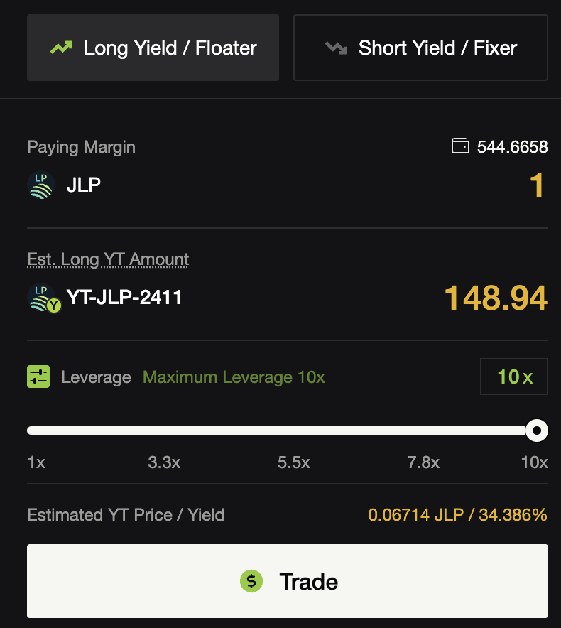
Currently, RateX can provide users with 10x leverage to trade YT-JLP.
In the JLP-2411 contract of the RateX test network (expiring at the end of November 24), a deposit of 1 JLP can buy 148.94 YT-JLP-2411.
Since the price of YT follows the following formula:
This is a non-linear formula that does not seem intuitive. When the implied yield is smaller, you can roughly assume that the rate of change of YT price is the same as the percentage change of Implied Yield (APY). (For example, for a contract with a six-month maturity, when the implied yield changes from 3% to 4%, the YT price change is about 4%/3%-1 = 33%. When it changes from 30% to 40%, the YT price change percentage is about 26%. There is a problem of sensitivity to the discount factor here). If you are a mature investor, we still recommend that you calculate it yourself for more accuracy. Here is a very detailed description of YT.
2. Fixed income investments
RateX constructs PT assets based on YT and ST, PT= 1-YT. Because YT is an asset whose value approaches 0 as it continues to receive yield, the value of PT will gradually approach a ST-JLP. If you choose to hold it until maturity, you will get a fixed income, which is itself a conservative passive income strategy.
You can also choose to do a PT spread strategy. If the YT price falls (implied yield decreases), the PT price will increase, and you can choose to redeem PT immediately to obtain a higher annualized return.
You can also choose a method similar to Kamino multiply, mortgaging PT to borrow funds to continue buying PT and generate higher returns. Of course, after adding leverage, you have to be careful about liquidation risks.
3. Arbitrage Trading
There is also a strategy based on predicting the APY arbitrage trading during the YT interest payment cycle. Since YT is a time-decaying asset, its value is amortized according to the implied yield. We will recalculate the value of YT at the end of each interest payment cycle. If the reduced value is not equal to the value of the yield you receive, then you have the opportunity to arbitrage by predicting APY data.
Suppose you buy a YT with an implied yield of 30%. At the next interest payment period, the implied yield is still 30%, and you receive an APY of 50%. However, the value of your YT decreases as the implied yield of 30% decreases over the remaining time.
This means that the yield you receive exceeds the reduction in the value of YT. If you can sell YT at the market price immediately, you have obtained an arbitrage opportunity by predicting the APY within this interest payment range. However, this short-term arbitrage opportunity is small, and the implied yield of YT reflects the expected average APY within the remaining period, so the failure of interest payment cycle arbitrage may become a source of profit for traders with longer-term strategies. Therefore, it is not recommended to participate unless you are a professional trader.
Original link


