


Preface
Continuing from the previous chapter, we publishedThe first article in the series Building a Powerful Crypto-Asset Portfolio Using Multi-Factor Strategies - Theoretical Basics, this article is the second article - data preprocessing.
Before/after calculating factor data, and before testing the validity of a single factor, the relevant data need to be processed. Specific data preprocessing involves the processing of duplicate values, outliers/missing values/extreme values, standardization and data frequency.
1. Duplicate values
Data related definitions:
Key: Represents a unique index. eg. For a piece of data with all tokens and all dates, the key is token_id/contract_address - date
Value: The object indexed by the key is called the value.
Diagnosing duplicate values first requires understanding what the data should look like. Usually the data is in the form of:
Time Series data. The key is time. eg. Five years of price data for a single token
Cross Section data (Cross Section). The key is individual. eg.2023.11.01 Price data of all tokens in the crypto market on that day
Panel data (Panel). The key is the combination of individual-time. For example. Price data of all tokens in the four years from 2019.01.01 to 2023.11.01.
Principle: Once the index (key) of the data is determined, you can know at what level the data should have no duplicate values.
Check method:
pd.DataFrame.duplicated(subset=[key 1, key 2, ...])
Check the number of duplicate values: pd.DataFrame.duplicated(subset=[key 1, key 2, ...]).sum()
Sampling to see duplicate samples: df[df.duplicated(subset=[...])].sample() After finding the sample, use df.loc to select all duplicate samples corresponding to the index
pd.merge(df 1, df 2, on=[key 1, key 2, ...], indicator=True, validate=1: 1)
In the horizontal merging function, adding the indicator parameter will generate the _merge field. Use dfm[_merge].value_counts() to check the number of samples from different sources after merging.
By adding the validate parameter, you can verify whether the index in the merged data set is as expected (1 to 1, 1 to many or many to many, the last case actually means no verification is required). If it is not as expected, the merge process will report an error and abort execution.
2. Outliers/missing values/extreme values
Common causes of outliers:
extreme case.For example, if the token price is 0.000001 $ or the token has a market value of only 500,000 US dollars, if it changes a little bit, there will be dozens of times of return.
Data characteristics.For example, if the token price data starts to be downloaded on January 1, 2020, then it is naturally impossible to calculate the return data on January 1, 2020, because there is no closing price of the previous day.
data error.Data providers will inevitably make mistakes, such as recording 12 yuan per token as 1.2 yuan per token.
Principles for handling outliers and missing values:
delete. Outliers that cannot reasonably be corrected or corrected may be considered for deletion.
replace. Usually used to process extreme values, such as winsorizing or taking logarithms (not commonly used).
filling. forMissing valuesYou can also consider filling in a reasonable way. Common ways includemean(or moving average),interpolation(Interpolation)、Fill in 0df.fillna(0), forward df.fillna(ffill)/backward filling df.fillna(bfill), etc. It is necessary to consider whether the assumptions on which the filling relies are consistent.
Use backward filling with caution in machine learning, as there is a risk of Look-ahead bias.
How to deal with extreme values:
1. Percentile method.
By arranging the order from small to large, data that exceeds the minimum and maximum ratios are replaced with critical data. For data with rich historical data, this method is relatively rough and not very applicable. Forcibly deleting a fixed proportion of data may cause a certain proportion of losses.
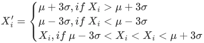
2.3σ / three standard deviation method
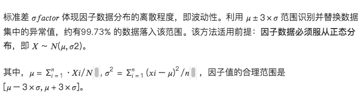
Make the following adjustments to all factors within the data range:
The disadvantage of this method is that commonly used data in the quantitative field, such as stock prices and token prices, often present a peaked and thick-tailed distribution, which does not conform to the assumption of normal distribution. In this case, using the 3 σ method will mistakenly identify a large amount of data as anomalies. value.
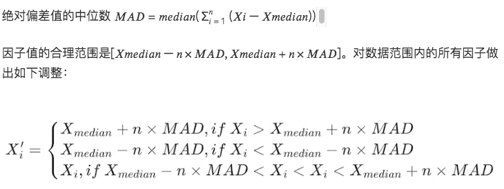
3. Median Absolute Deviation (MAD) method
This method is based on the median and absolute deviation, making the processed data less sensitive to extreme values or outliers. More robust than methods based on mean and standard deviation.
# Handle extreme value situations of factor data
class Extreme(object):
def __init__(s, ini_data):
s.ini_data = ini_data
def three_sigma(s, n= 3):
mean = s.ini_data.mean()
std = s.ini_data.std()
low = mean - n*std
high = mean + n*std
return np.clip(s.ini_data, low, high)
def mad(s, n= 3):
median = s.ini_data.median()
mad_median = abs(s.ini_data - median).median()
high = median + n * mad_median
low = median - n * mad_median
return np.clip(s.ini_data, low, high)
def quantile(s, l = 0.025, h = 0.975):
low = s.ini_data.quantile(l)
high = s.ini_data.quantile(h)
return np.clip(s.ini_data, low, high)
3. Standardization
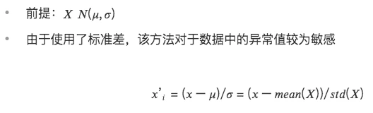
1.Z-score standardization
2. Maximum and minimum value difference standardization (Min-Max Scaling)
Converts each factor data into data in the (0, 1) interval, allowing comparison of data of different sizes or ranges, but it does not change the distribution within the data, nor does it cause the sum to become 1.
Due to considering the maximum and minimum values, it is sensitive to outliers
Unifying the dimensions facilitates comparison of data in different dimensions.
3. Rank Scaling
Convert data features into their rankings, and convert these rankings into scores between 0 and 1, typically their percentiles in the data set. *
This method is insensitive to outliers since rankings are not affected by outliers.
Absolute distances between points in the data are not maintained, but converted to relative rankings.


# Standardized factor data class Scale(object):
def __init__(s, ini_data, date):
s.ini_data = ini_data
s.date = date
def zscore(s):
mean = s.ini_data.mean()
std = s.ini_data.std()
return s.ini_data.sub(mean).div(std)
def maxmin(s):
min = s.ini_data.min()
max = s.ini_data.max()
return s.ini_data.sub(min).div(max - min)
def normRank(s):
# Rank the specified column, method=min means that the same value will have the same ranking, not the average ranking
ranks = s.ini_data.rank(method=min)
return ranks.div(ranks.max())
4. Data frequency
Sometimes the data obtained is not of the frequency required for our analysis. For example, if the level of analysis is monthly and the frequency of original data is daily, you need to use downsampling, that is, the aggregated data is monthly.
Downsampling
RefersAggregate data in a collection into one row of data, for example, daily data is aggregated into monthly data. At this time, the characteristics of each aggregated indicator need to be considered. Common operations include:
first value/last value
mean/median
standard deviation
upsampling
It refers to splitting one row of data into multiple rows of data, such as annual data used for monthly analysis. This situation usually requires simple repetition, and sometimes it is necessary to aggregate the annual data into each month in proportion.


